VA-FDTD

SHAPE MODELER

VA-FDTD is introduced using a simple vibroacoustic analysis example. The vibration response and acoustic radiation of an aluminum plate floating in a box filled with air is analysed. For more details, please refer to the help of each software.

Click image to zoom up

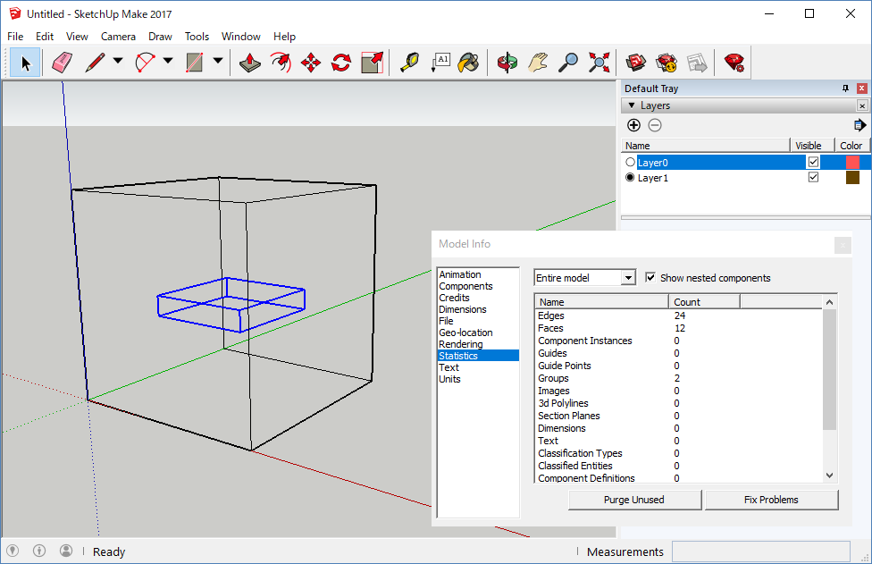
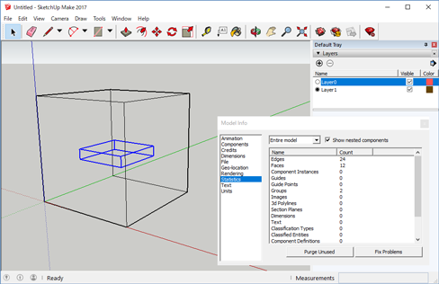
• First, create the geometry to be analysed using a CAD software. In this tutorial, SketchUp Make 2017 with the plugin is employed. Launch SketchUp and select "Architectural Design - Millimeters" as the template. If a person is displayed, click the person and delete it with the DELETE key, open Window > Model Info > Statistics, and click "Purge Unused".
• Click the "Shapes" button on the toolbar then click at the origin and move your mouse slightly (do not drag). Enter "1000mm, 1000mm" and press the ENTER key to draw a square of size 1000x1000mm^2. Next, click the "Push/Pull" button on the toolbar. Click the square drawn earlier and move your mouse slightly (do not drag). Enter "1000mm" and press the ENTER key, then the square is stretched upward and a cube is created.
• Next, click the "Select" button on the toolbar. Drag the mouse in such a way that the entire cube is included to select the cube. Right-click on the cube and click "Make Group" to have the cube as one part.
• Open Window > Default Tray > Layer, press the "+" button to create a new layer, and set the layer name "Layer1". Check the radio button of "Layer1" and uncheck "Visible" of "Layer0".
• Click the "Shapes" button on the toolbar. Click the origin and move your mouse slightly (do not drag). Enter "500mm, 500mm" and press the ENTER key, then a square is drawn. Next, click the "push/pull" button on the toolbar. Click the square drawn earlier and move your mouse slightly (do not drag). Enter "100mm" and press the ENTER key, the square is stretched upward and a rectangular parallelepiped is created.
• Next, click the "Select" button on the toolbar. Drag the mouse in such a way that the entire rectangular parallelepiped is selected then right-click on the cube and click "Make Group".
• Click the "Move" button on the toolbar. Click on the top of the rectangular parallelepiped and move your mouse slightly in parallel with the red axis (do not drag). Enter "250mm" and press the ENTER key, then the rectangular parallelepiped moves in the red axis direction. In the same way, move 250mm with the green axis and 400mm with the blue axis.
• Check "Visible" of "Layer1" and click View > Face Style > Wireframe.
• Click File > Export DXF for VA-FDTD, select "Millimeters" as Export units, and save the shapes as the DXF file in the appropriate directory.

VA-FDTD INTERFACE

The procedure to set analysis configurations using VA-FDTD INTERFACE is described in what follows.

Click image to zoom up

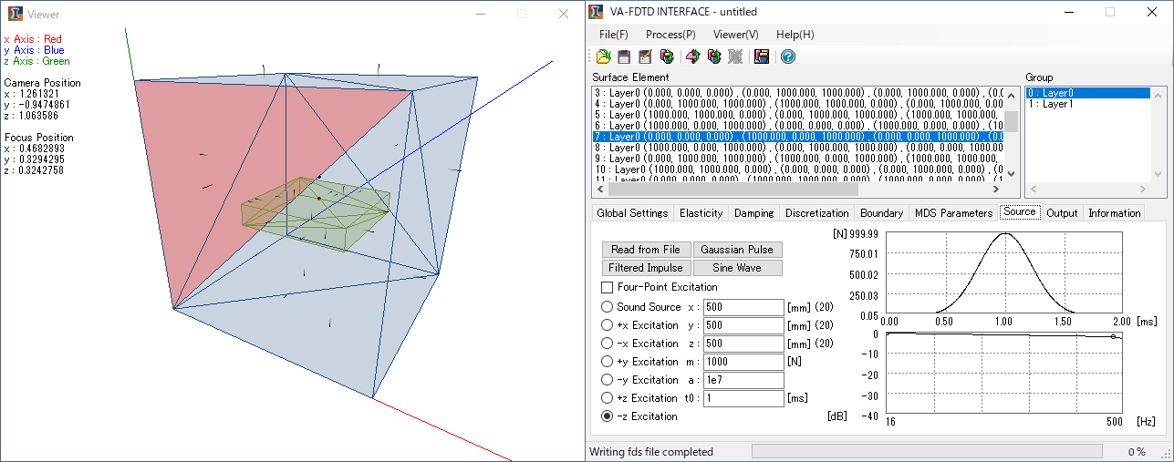
• Launch VA-FDTD INTERFACE and click the "Import" button on the tool bar. Indicate the DXF file you just exported, then the Import Configuration dialog will open. Set Round Setting to "1mm" (round off less than 1mm), uncheck the box of "Ignore ...", and click the OK button. Click the "Viewer" button on the toolbar to display the shapes. Check that the cube and the rectangular parallelepiped created by the shape modeler are correctly displayed. Additionally, make sure that the normal for all of the surfaces are outward with respect to the shapes to be analysed.
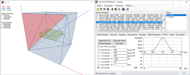
• The configuration setting will proceed in order from the leftmost tab of VA-FDTD INTERFACE.
• On the Global Settings tab, you can set the units and the target frequency range. In this tutorial, set Maximum of Target Frequency Range to "500"[Hz].
• On the Elasticity tab, you can set the media that fill the shapes to be analysed. In this tutorial, click "0: Layer0" in the Group list, and then, select "Air" from the Material combo box. In the same way, set "1: Layer1" to "Aluminum".
• On the Damping tab, you can set the damping. For this example, the media are assumed to be lossless, so this step can be skipped.
• On the Discretization tab, you can set the discretization conditions. This tutorial employs 25[mm] as the spatial interval which is sufficiently small to analyse the space up to 500[Hz] and can divide 1000[mm] without gaps. In the Spatial Step, enter "0"[mm] for Start Position, "1000"[mm] for End Position, and "25"[mm] for Interval. Make sure that the "x" radio button is checked and click the "Add" button. Next, check the "y" radio button, click the "Add" button, check the "z" radio button, and click the "Add" button. Information on the spatial discretization for each axis is listed in the combo box on the left of the xyz radio buttons. Confirm the information. After the spatial discretization setting is completed, the maximum time interval derived from the stability condition is displayed. Click the "Set Maximum Time Interval" button to set the time interval to the maximum value. Finally, set Maximum Time to "5"[ms].
• On the Boundary tab, you can set the boundary conditions. In this tutorial, click "0: Layer0" in the Group list and check the "Fixed Boundary" radio button.
• On the MDS Parameters tab, you can search for parameters when Mass-Damper-Spring Boundaries are selected as the boundary condition. For this example, this step can be skipped.
• On the Source tab, you can set the excitation condition. Click the "Gaussian Pulse" button. Check the "-z Excitation" radio button and set x, y, and z to "500"[mm], respectively. Next, set m to "1000"[N], a to "1e7", and t0 to "1"[ms].
• On the Output tab, you can set the output conditions. Make sure the "MATLAB + ParaView" radio button is checked. Next, confirm that the "yz" radio button on MATLAB Target Surface is checked. Enter "500"[mm] for Position and click the "Add" button. In the combo box, the cross-sections to be output are listed. Confirm the information and enter "20" for Frame. Next, make sure that the "p" radio button of MATLAB Receiving Point is checked, enter "500", "500", and "600" [mm] in x, y, and z Positions, respectively, and click the "Add" button. In the combo box, the points where the responses will be output are listed. Confirm the information. Finally, for ParaView parameters, enter "20" for Frame and "2000" to Ratio.
• After all the above settings are completed, click the "Save as ..." button on the toolbar and save the information file (FDI file) with a suitable file name. Next, click the "Export" button on the toolbar and indicate a directory for output of the configuration file (FDC file). After the output is completed, the Export fds File dialog opens. Click "Yes" to export the shape file (FDS file).

VA-FDTD CHECKER

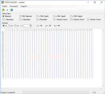
Check whether the spatial discretization information and the boundary settings were exported correctly using VA-FDTD CHECKER.

Click image to zoom up

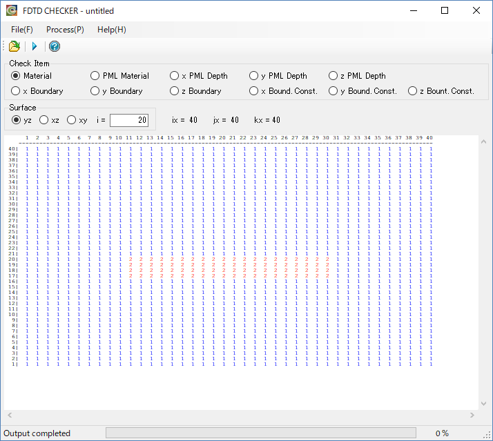
• Launch VA-FDTD CHECKER and click the "Open" button on the tool bar. Select the FDC file you have exported, then the spatial discretization information and the boundary settings will be loaded.
• Confirm that the "Material" radio button of Check Item and the "yz" radio button of Surface are checked, and enter "20" for i= of Surface. Click the "Check" button on the toolbar, then the medium number distribution in the yz plane at the x-directional spatial step of 20 is displayed. Here "1" means the first group (0: Layer0) and "2" means the second one (1: Layer1) of the Group list in VA-FDTD INTERFACE.
• Check the "y Boundary" radio button of Check Item and click the "Check" button on the tool bar to display the y-directional boundary condition number distribution in the yz plane at the x-directional spatial step of 20. Here, "-2" means the left-side fixed boundary and "2" the right-side fixed boundary. Check the "z Boundary" radio button of Check Item and click the "Check" button on the toolbar to display the z-directional boundary condition number distribution in the yz plane at the x-directional spatial step of 20. Here, "-2" means the lower-side fixed boundary and "2" the upper-side fixed boundary. Check the "x Boundary" radio button of Check Item and enter "1" for i= of Surface. Click the "Check" button on the toolbar, then the x-directional boundary condition number distribution in the yz plane at the x-directional spatial step of 1. Here, "-2" means the front-side fixed boundary.
• If the distributions are not correct, return to VA-FDTD INTERFACE and reconfirm the settings (especially the direction of the surface normals).

VA-FDTD SOLVER

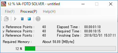
Run the FDTD calculation and export the results using VA-FDTD SOLVER.

Click image to zoom up

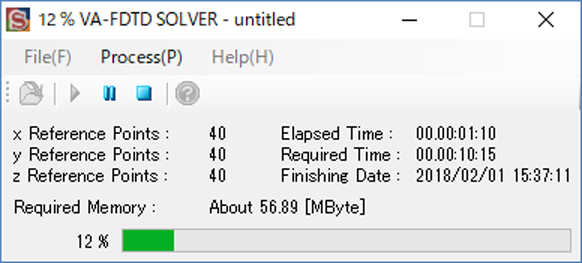
• Launch VA-FDTD SOLVER and click the "Open" button on the toolbar. Indicate the FDS file exported with VA-FDTD INTERFACE, and then all required settings are loaded.
• Click the "Start" button on the toolbar and indicate the directory you want to export the calculated results.
• Click the "Pause" button on the toolbar if you want to pause the calculation halfway, or click the "Abort" button on the toolbar if you want to abort it.
• A completion message will be displayed at the bottom when the calculation is completed.

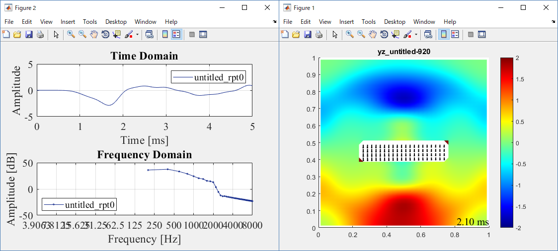
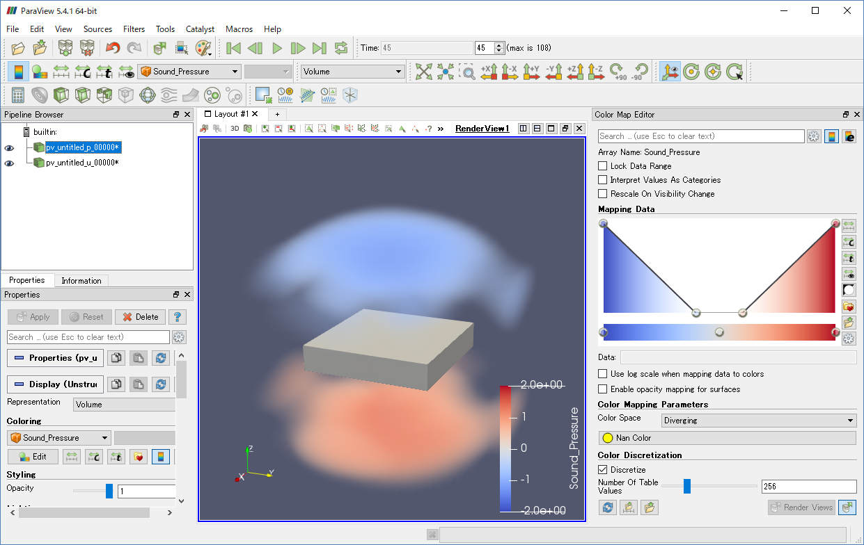
RESULT VIEWER

Visualize the calculated results using MATLAB and ParaView.

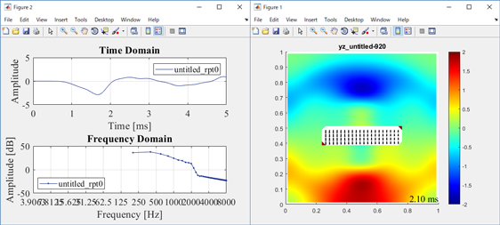
Click image to zoom up

• Copy the MATLAB FUNCTION M-FILES to the directory included in the search paths of MATLAB.
• Launch MATLAB and move to the directory that contains the calculated results output by VA-FDTD SOLVER.
• Enter "vafdtd_graph('***','rpt0');" (*** is a part of the file name such as ***.fds), then the waveform at the sound receiving point set by VA-FDTD INTERFACE is displayed. Additionally, enter "vafdtd_animation(0,'***',-2,2,2000,20);", then the animation of the cross-sectional distribution set by VA-FDTD INTERFACE is displayed.

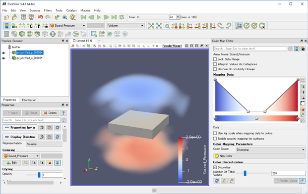
Click image to zoom up

• Launch ParaView and click the "Open" button on the toolbar. Indicate "pv_***_p_..vtk" in the directory that includes the calculated results and click the "Apply" button of Properties.
• Click "Rescale to Custom Data Range" on the toolbar and enter "-2" for Minimum and "2" for Maximum.
• Click "Edit Color Map" on the tool bar, set Mapping Data as shown above, and change Presentation of Toolbar to "Volume".
• Next, click "Open" button on the tool bar and indicate "pv_***_u_..vtk", and click the "Apply" button of Properties.
• Click the "Play" button to view the 3D animation.